We’re excited to announce that Visidon will be exhibiting at the Embedded Vision Summit (EVS) in Santa Clara, May 11–13, 2026!

At this year’s event, we’re showcasing three live demos of AI-powered video enhancement, all running in real time on embedded platforms: low-light restoration in the RAW domain on Qualcomm, face super-resolution for long-range imaging and video conferencing, and a traffic enhancement module running on NVIDIA Tegra.

Live Demos at Our Booth

We’ll be showcasing three live demonstrations highlighting our latest innovations:

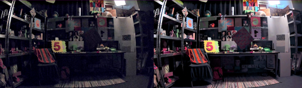
AI Low-Light Enhancement (RAW Domain, Real-Time on Qualcomm)
Our core embedded video technology operates directly in the RAW domain, enabling superior restoration before ISP processing. Running in real time on a Qualcomm platform, it delivers clean, sharp video with accurate colors—even in extremely low-light conditions.

To demonstrate its capabilities, we’re using a lightbox setup with minimal lighting, specifically designed to highlight performance in ultra low-light conditions and scenes with camera motion.

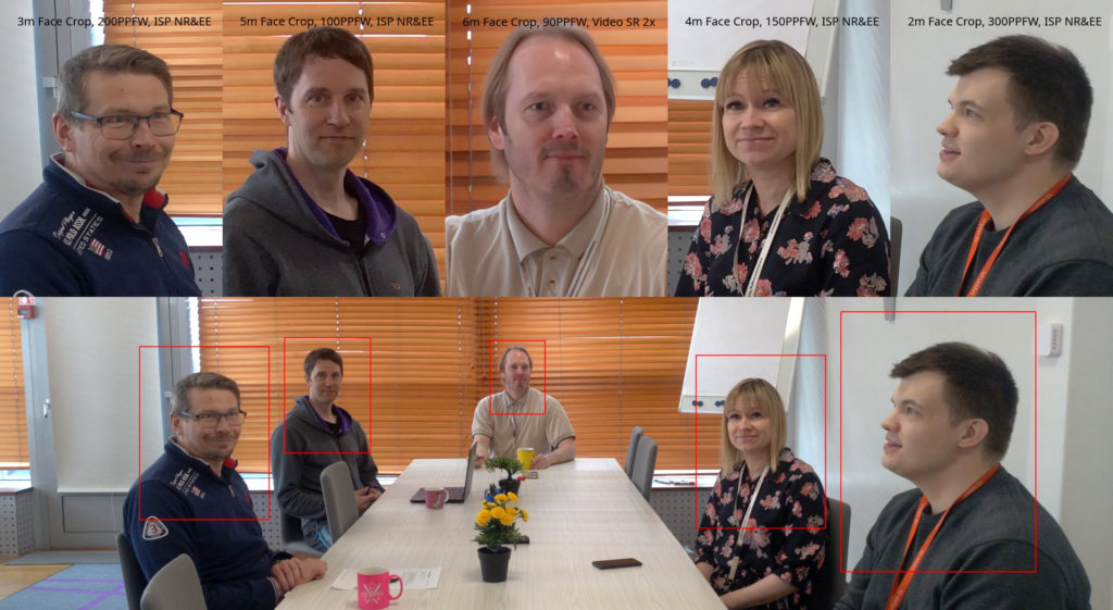
Video Face Super Resolution
This solution uses a dedicated deep learning model trained for facial reconstruction. It enhances facial regions frame by frame, restoring fine details while maintaining identity consistency and temporal stability.

The result is clear, natural-looking faces even at long distances, making it ideal for video conferencing and multi-person scenes. Read more from our previous blog here.

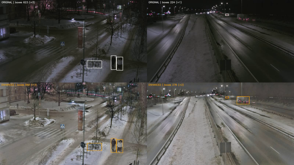
Visidon Traffic Image Booster
Designed for intelligent transportation and surveillance applications, this lightweight enhancement module operates on processed video streams. It improves visibility in challenging conditions such as low light, adverse weather, and long-range capture—without requiring changes to the existing camera pipeline.

By enhancing image quality at the source, it significantly boosts downstream analytics like object detection and traffic monitoring. It integrates seamlessly into existing pipelines and is optimized for platforms such as NVIDIA Tegra.

Join us at EVS 2026

Experience our technology live at the Embedded Vision Summit, Booth 604.

Want to attend?
Register here: https://embeddedvisionsummit.com/

• Free Exhibits-Only Pass: email sales@visidon.fi
• Discount on full conference passes: use code 26EVSUM-PARTNER at embeddedvisionsummit.com

Let’s meet at EVS and talk more!

Keywords: #EVS26 AI, CNN, denoising algorithms, RAW denoise, YUV denoise, RAW denoising, YUV denoising, low-light enhancement, embedded camera systems, real-time video enhancement.